Differentiable ML for Lake-Ice Modeling

I had a long conversation with Claude working through the mechanics of “differentiable modeling” — trusted physics (a physics component) fused with learnable neural-network closures, trained end-to-end by gradient descent. This is directly relevant to a MOSART river/lake-ice scheme I’m thinking about, so instead of letting the conversation disappear into scrollback, I asked Claude to turn it into a self-contained reference built from three worked examples, and I’m migrating that write-up here. The text below is Claude’s draft, lightly edited by me (mostly to drop some jargon). Every number is reproduced exactly by the companion notebook (linked at the bottom) with fixed random seeds, and every figure is generated from the same fixed-seed code.

Overview — what is differentiable ML, and why do we need it?

The problem with the two extremes

Environmental systems like lake ice sit between two modeling styles that each fail in a different way:

Pure physics models encode what we understand (energy balance, Stefan’s ice-growth law) but contain empirical closures — coefficients and sub-rules that nobody can derive from first principles (how snow insulation slows ice growth, how wind redistributes heat). These are usually hand-tuned or calibrated one constant at a time.
Pure machine-learning models (a neural network mapping inputs straight to ice thickness) can fit anything, but they ignore the physics we do trust, need enormous data, and extrapolate poorly outside their training range — a fatal flaw for climate projection, where the future is by definition out-of-sample.

Differentiable modeling is the fusion: keep the physical structure you trust as a differentiable physics component, and replace only the uncertain empirical closures with learnable functions (small neural networks). Because the entire model — physics and networks — is written in an autodiff framework (PyTorch, JAX), gradients of a loss with respect to every network weight can be computed through the physics, and the whole thing is trained together, end-to-end.

Why “differentiable” specifically?

The word means one concrete thing: the model is built entirely from operations whose derivatives are known and composable, so the chain rule can propagate a single loss gradient from the output all the way back to every internal parameter in one pass. That is what lets a neural closure buried inside a physical model learn from a loss defined on the model’s final output (observed ice thickness, breakup date) rather than needing direct observations of the closure itself (which usually do not exist — nobody measures “the Stefan coefficient”).

Why the nonlinearity matters (physics + NN)

If the world were linear, none of this would be necessary — you could fit a single global slope. The reason we need a nonlinear closure (the NN) wrapped in nonlinear physics (the \(\sqrt{FDD}\) law) is that the real dependencies are curved and interacting: snow’s effect on ice growth is not a constant offset, it modulates the rate at which cold air grows ice. The deeper questions below show concretely that this interaction — multiplicative, not additive — is exactly why the physics and the network must be trained jointly rather than in sequence.

The physics anchor used throughout

Every example below is built on Stefan’s law, the classical lake- and sea-ice thickness relationship:

\[h = \alpha \sqrt{FDD}\]

symbol	meaning	units
`h`	ice thickness	cm
\(FDD\)	accumulated freezing-degree-days (the cold forcing)	°C·day
\(\alpha\)	Stefan coefficient — lumps snow, wind, water heat flux	cm · (°C·day)^(−1/2)

\(\sqrt{FDD}\) is the trusted physics component. \(\alpha\) is the closure — a fixed constant in Example 1, a single calibrated parameter in Example 2, and a learned function \(\alpha(\text{snow})\) in Example 3.

Example 1 — Autodiff sanity check (no learning yet)

Before I trust an autodiff engine to train anything, I want to see it reproduce a derivative I can check by hand. So this first example does no learning at all — it’s just a unit test on the gradient machinery.


Problem	Confirm the autodiff engine reproduces the exact textbook derivative of Stefan’s law.
Known	\(\alpha\) = 3.0 (fixed constant); \(FDD\) swept 1→400.
Unknown	Nothing. This is a differentiation-engine unit test.
Goal	Verify \(\partial h/\partial FDD\) from `.backward()` equals the calculus answer \(\alpha/(2\sqrt{FDD})\).
What diffML is doing	Nothing yet — establishing that the gradient engine is trustworthy before we rely on it.

alpha_true = 3.0
FDD = torch.linspace(1, 400, 200, requires_grad=True)
h = alpha_true * torch.sqrt(FDD)          # forward pass
h.sum().backward()                         # backward pass -> FDD.grad
analytic = alpha_true / (2*torch.sqrt(FDD))

Result — autodiff equals calculus to floating-point precision:

\(FDD\)	\(\partial h/\partial FDD\) autodiff	\(\alpha/(2\sqrt{FDD})\) calculus
1	1.500000	1.500000
100	0.150569	0.150000

Maximum absolute error across all 200 points: 5.96e-08. Autodiff is the chain rule executed exactly — not a finite-difference approximation. Everything else stands on this.

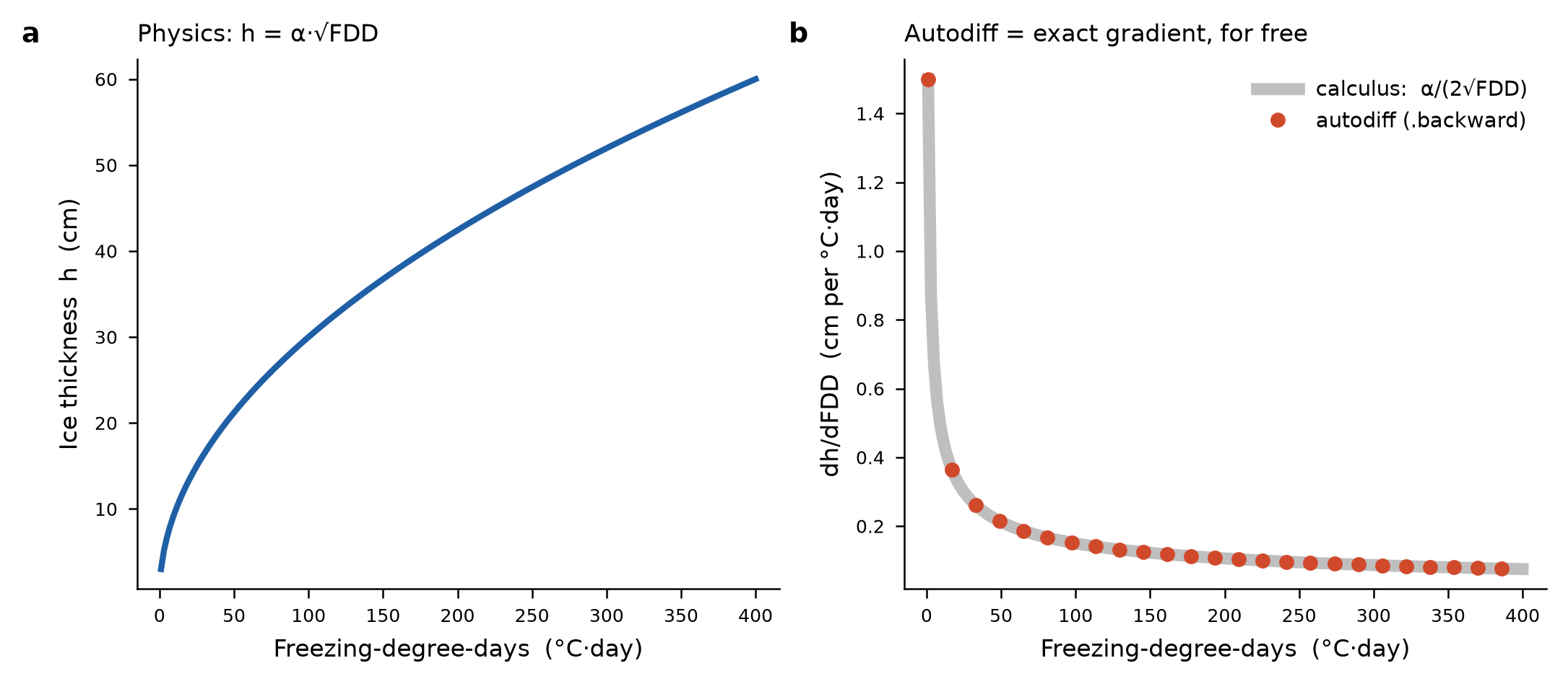
Example 1: autodiff gradient overlaid on the analytic derivative curve

Figure 1. Autodiff sanity check. The gradient \(\partial h/\partial FDD\) returned by .backward() (markers) lies exactly on the analytic curve \(\alpha/(2\sqrt{FDD})\) (line) across the full \(FDD\) sweep. Maximum absolute error over all 200 points is 5.96e-08 — autodiff executes the chain rule exactly, not as a finite-difference approximation.

Example 2 — One-parameter calibration by gradient descent

Now the first bit of actual learning. Nothing changes about the physics — I just stop pretending I know \(\alpha\) and let gradient descent find it from noisy data. This is calibration, the thing hydrologists already do with SCE-UA all day; the only twist is that the gradient tells me which way to step.


Problem	Recover the single best \(\alpha\) from noisy ice-thickness observations.
Known	\(FDD_{obs}\) and noisy \(h_{obs}\) — the data (same “known input” role \(FDD\) played in Ex. 1).
Unknown	\(\alpha\) — promoted from fixed constant to a trainable parameter (`requires_grad=True`).
Goal	Minimize mean-squared error between \(\alpha\sqrt{FDD}\) and \(h_{obs}\).
What diffML is doing	Using \(\partial \text{Loss}/\partial \alpha\) to walk \(\alpha\) downhill — the same job SCE-UA does in calibration, but gradient-guided instead of population-search.

The only thing that changed from Example 1 is \(\alpha\)’s status: known constant → unknown to be found. The computation graph is \(\alpha \;\to\; \text{pred} = \alpha\sqrt{FDD} \;\to\; \text{diff} = \text{pred}-h_{obs} \;\to\; \text{sq} = \text{diff}^2 \;\to\; \text{loss} = \text{mean}(\text{sq})\).

The forward pass, in numbers (starting guess \(\alpha\) = 1.0)

First four of the 30 data points:

\(FDD\)	\(\sqrt{FDD}\)	pred = \(\alpha\sqrt{FDD}\)	\(h_{obs}\)	diff	sq = diff²
20.0	4.472	4.472	11.728	-7.256	52.64
32.4	5.693	5.693	15.351	-9.658	93.28
44.8	6.695	6.695	19.710	-13.015	169.39
57.2	7.566	7.566	22.047	-14.481	209.69

Summing all 30 squared residuals gives 23988.48, so loss = 23988.48 / 30 = 799.6161 — matching loss.item() exactly.

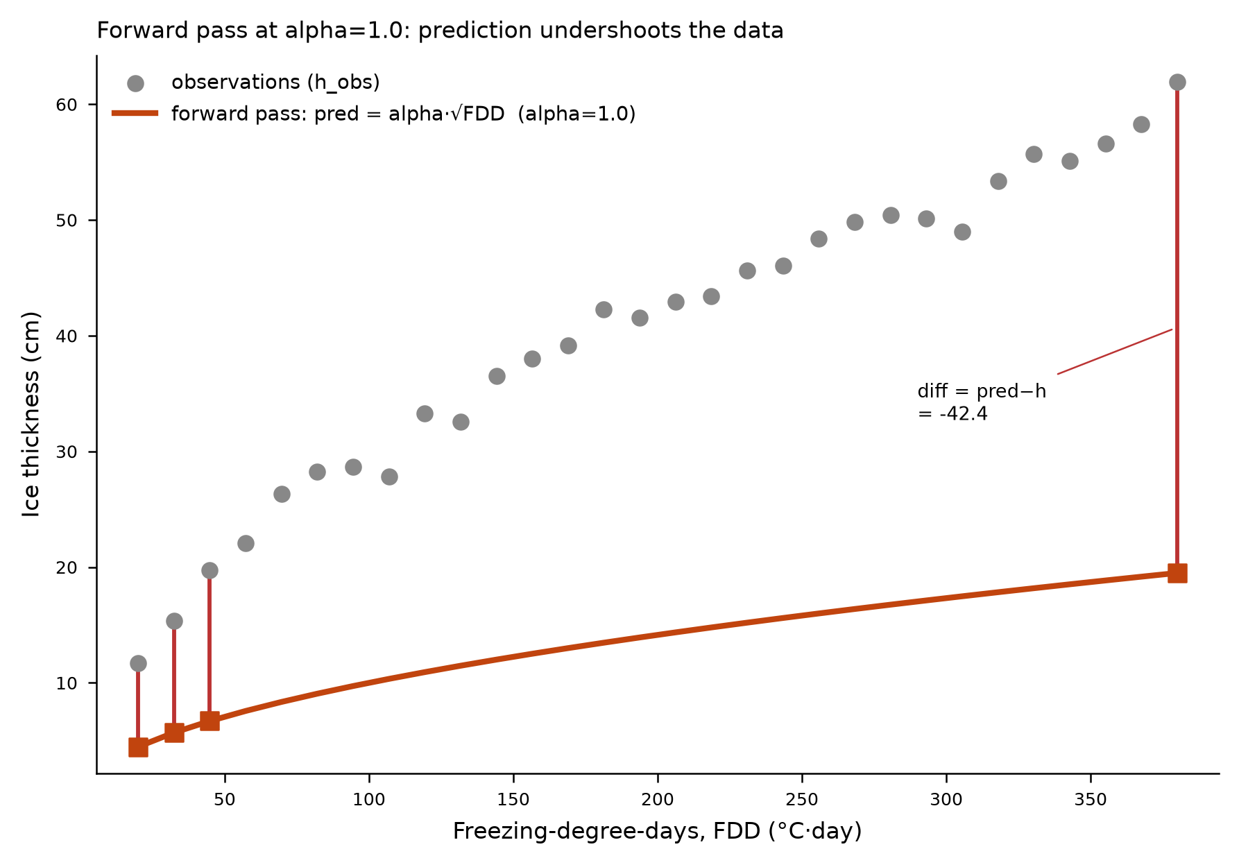
Example 2 forward pass: prediction undershooting the observations

Figure 2. Example 2 forward pass at the starting guess \(\alpha\) = 1.0. The prediction line \(\alpha\sqrt{FDD}\) sits well below the noisy observations; vertical segments mark the residuals \(\text{pred} - h_{obs}\) whose squares sum to 23988.48, giving the initial loss of 799.6161. The systematic undershoot is what the negative gradient will correct.

The backward pass, derived by hand

Walk the four links of the chain rule, each verified against PyTorch’s retained gradients:

link	local derivative
\(\partial \text{loss}/\partial \text{sq}\)	`1/N`
\(\partial \text{sq}/\partial \text{diff}\)	`2·diff`
\(\partial \text{diff}/\partial \text{pred}\)	`1`
\(\partial \text{pred}/\partial \alpha\)	\(\sqrt{FDD}\)

Multiplying and summing across all points collapses to the closed form:

\[\frac{\partial Loss}{\partial \alpha} = \frac{2}{N}\sum_i \sqrt{FDD_i}\,\bigl(\alpha\sqrt{FDD_i} - h_i\bigr)\]

At \(\alpha\) = 1.0 this evaluates to:

	value
\(\partial \text{Loss}/\partial \alpha\) — autograd (`.backward()`)	-798.8566
\(\partial \text{Loss}/\partial \alpha\) — closed form (by hand)	-798.8566

Identical. The negative sign says “\(\alpha\) is too small — increase it,” which is correct (true \(\alpha\) = 3.0).

Direction and step size

Direction = the sign of the gradient. Scanning \(\alpha\) = 1,2,3,4,5, the gradient flips sign exactly at the true \(\alpha\) = 3.0 — that zero-crossing is the minimum.
Step size in plain SGD is literally lr·grad, so it shrinks naturally as the gradient flattens near the minimum. The Adam optimizer used here instead normalizes the step by a running RMS of the gradient (\(m̂/√v̂\)), which is why one fixed lr=0.1 works across a ~1000× range of gradient magnitudes over the run, and why \(\alpha\) overshoots to ~3.26 near step 35 (momentum) before settling. Final recovered value: \(\alpha\) = 2.9971 (true 3.0).

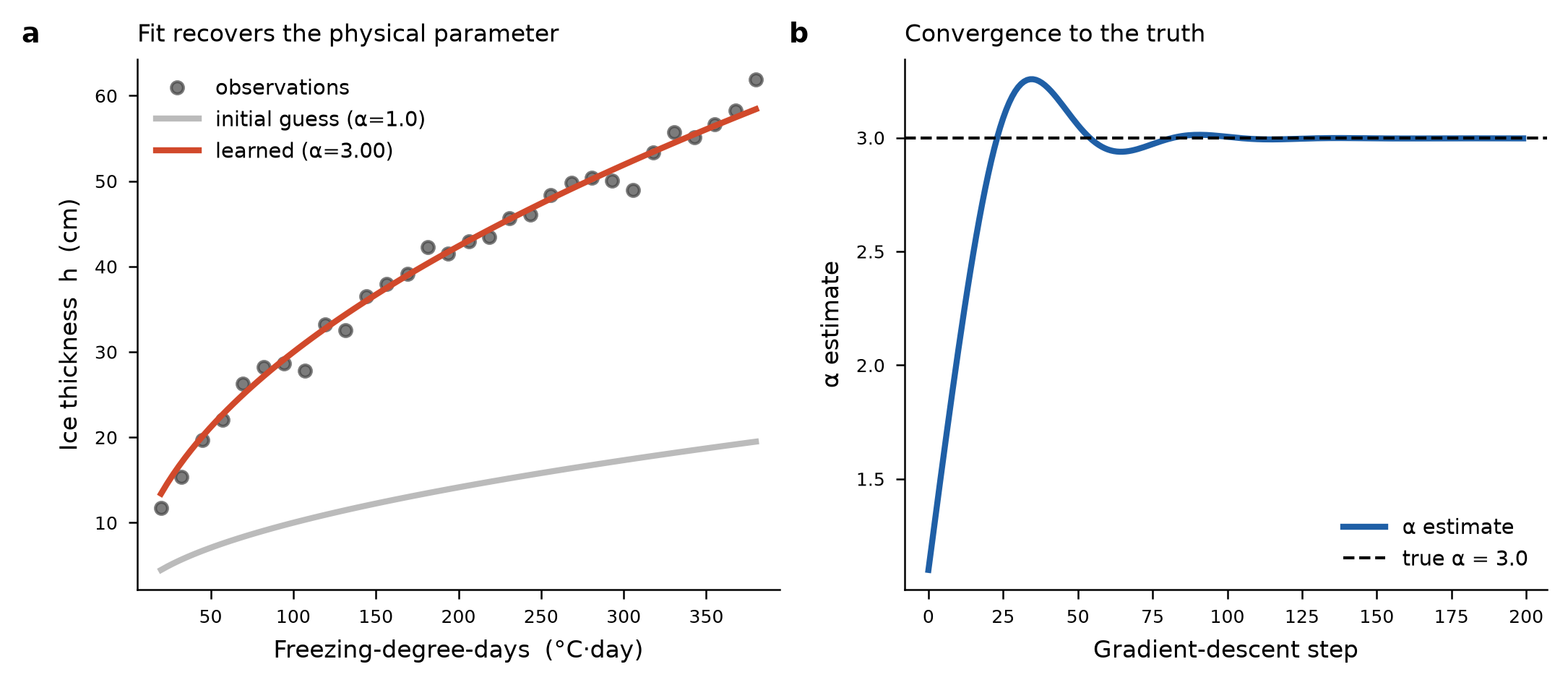
Example 2 calibration: alpha trace converging to 3.0

Figure 3. One-parameter calibration by gradient descent. Left: the \(\alpha\) trajectory over 200 Adam steps, climbing from 1.0, overshooting to ~3.26 near step 35 (momentum), then settling at the recovered value 2.9971 (true \(\alpha\) = 3.0, dashed). Right: the fitted Stefan curve through the observations at the converged \(\alpha\).

Calibration note: for a single scalar like this, derivative-free global search (SCE-UA, DDS) converges about as well as gradient descent and is arguably more robust (global vs. local). Differentiability’s advantage only becomes decisive when the number of parameters grows — which is exactly Example 3’s regime, and is quantified in the “three ways to train” section below.

Example 3 — Hybrid ML: a network learns an unknown closure inside fixed physics

This is the one that made the whole idea click for me. Here \(\alpha\) isn’t a constant anymore — it depends on snow cover through a rule I deliberately hide from the model. The network never sees \(\alpha\) at all, only noisy ice thickness, and it has to recover the closure by working through the physics I keep fixed. If that works, it’s the toy version of exactly what I want to do in MOSART.


Problem	\(\alpha\) is not constant — it depends on snow cover. We do not know the form \(\alpha(\text{snow})\). Learn it while keeping \(\sqrt{FDD}\) physics fixed.
Known to the model	`snow` (fed into the NN) and \(FDD\) (kept in the fixed physics term).
Hidden	The rule \(\alpha = 3.5 - 1.8\cdot\text{snow}\) is never shown to the network. \(\alpha\) itself appears nowhere in the data — only noisy \(h_{data}\) does.
Goal	Recover \(\alpha(\text{snow})\) purely from residual structure in \(h_{data}\), trusting the physics.
What diffML is doing	Gradients flow from the loss, through the fixed physics, into the NN weights — the network discovers \(\alpha(\text{snow})\) jointly with how it interacts with \(FDD\).

Architecture: \(\text{snow} \;\to\; \text{Linear}(1,16) \;\to\; \text{Tanh} \;\to\; \text{Linear}(16,16) \;\to\; \text{Tanh} \;\to\; \text{Linear}(16,1) \;\to\; \text{Softplus} \;\to\; \alpha\). The Tanh layers provide expressiveness (the “neural-network basics” section below explains why they are essential); the final Softplus forces \(\alpha\) > 0, since a negative Stefan coefficient is unphysical. The network has 321 learnable parameters.

alpha_pred = net(snow_d[:, None]).squeeze(1)   # NN: snow -> alpha
h_pred = alpha_pred * torch.sqrt(FDD_d)         # physics retained (multiplicative)
loss = ((h_pred - h_data)**2).mean()
loss.backward()                                  # gradient: loss -> physics -> NN weights

Result — the network recovers the hidden rule to within ~0.01 across the whole snow range:

snow	\(\alpha\) true = 3.5 − 1.8·snow	\(\alpha\) recovered (NN)	error
0.00	3.500	3.511	+0.011
0.25	3.050	3.037	-0.013
0.50	2.600	2.602	+0.002
0.75	2.150	2.158	+0.008
1.00	1.700	1.707	+0.007

Overall fit RMSE = 1.624 cm, essentially the noise floor (1.5 cm). The network learned a closure it was never directly shown, purely from the residual structure the trusted physics left behind.

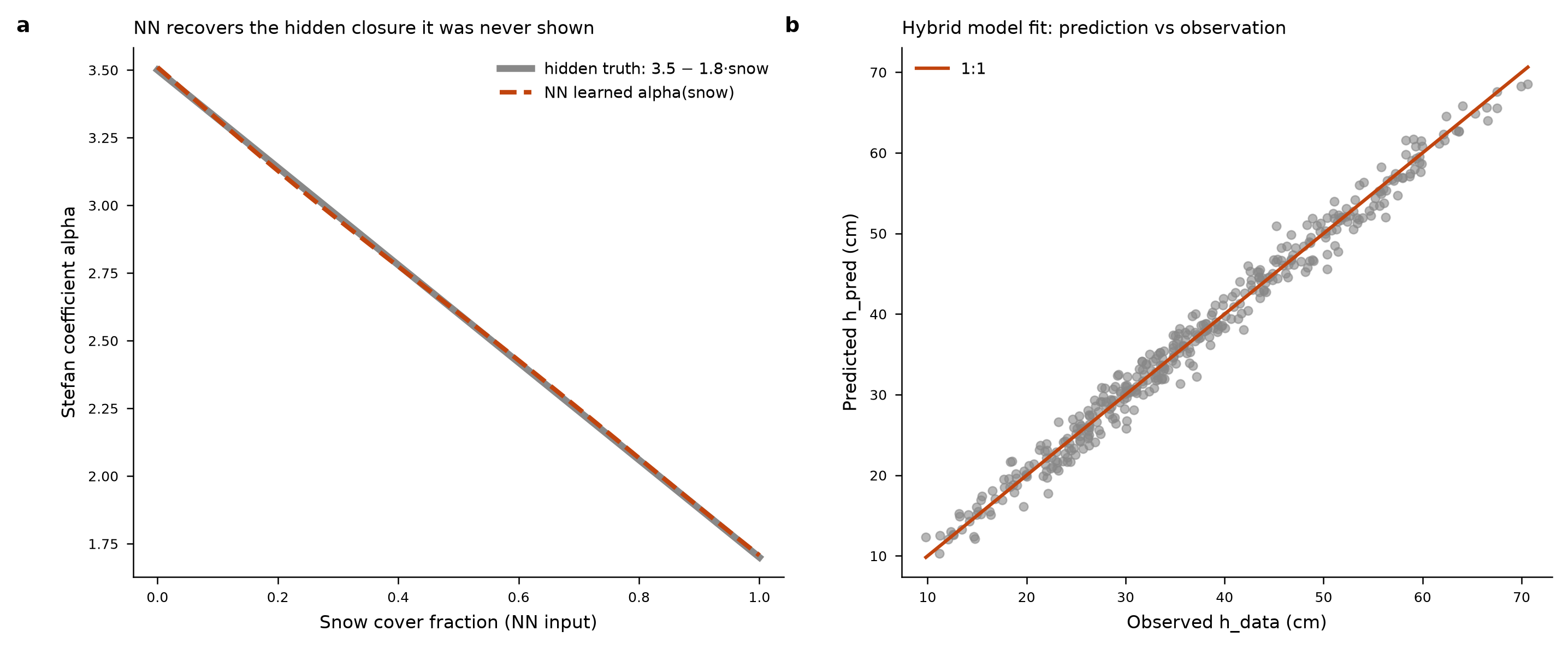
Example 3: NN-recovered alpha(snow) overlaying the hidden truth line

Figure 4. Hybrid ML recovering an unknown closure. Left: the network’s learned \(\alpha(\text{snow})\) (curve) overlays the hidden truth \(\alpha = 3.5 - 1.8\cdot\text{snow}\) (dashed) to within ~0.01 everywhere, despite \(\alpha\) never appearing in the training data. Right: predicted vs. observed ice thickness, RMSE 1.624 cm — essentially the 1.5 cm noise floor.

Deeper questions I kept poking at

The three examples above are the clean story. But every time I thought I understood it, I found a “wait, but why can’t I just…” question, and chasing those down is where I actually learned something. These are the four that stuck.

3a. Why not split it? Run the physics first, then a separate residual network

This was my first instinct, and it’s probably yours too: since snow isn’t part of the physics component, why bother training jointly? Why not (1) run the physics component once with a fixed average \(\alpha_0\), (2) compute \(\text{residual} = h_{data} - \alpha_0\sqrt{FDD}\), and (3) train a separate network NN(snow) to fit that residual? I had Claude build exactly that and compare:

approach	RMSE (cm)
Noise floor (irreducible)	1.50
Stage-wise: fixed \(\alpha_0\) = 2.6, additive NN(snow) → residual	2.66
End-to-end: NN(snow) → \(\alpha\), multiplies \(\sqrt{FDD}\)	1.62

The stage-wise split leaves nearly double the residual error. The reason is that the true process is multiplicative — \(\alpha\) multiplies \(\sqrt{FDD}\) — not additive. When you fix \(\alpha_0\) and subtract, the leftover residual is not a clean function of snow alone: it still carries an \(FDD\)-shaped error, because \(\alpha_0\) is wrong by a different amount at every snow value. Holding snow fixed near 0 (where \(\alpha_0\) = 2.6 is most wrong) and looking at how that residual varies with \(FDD\):

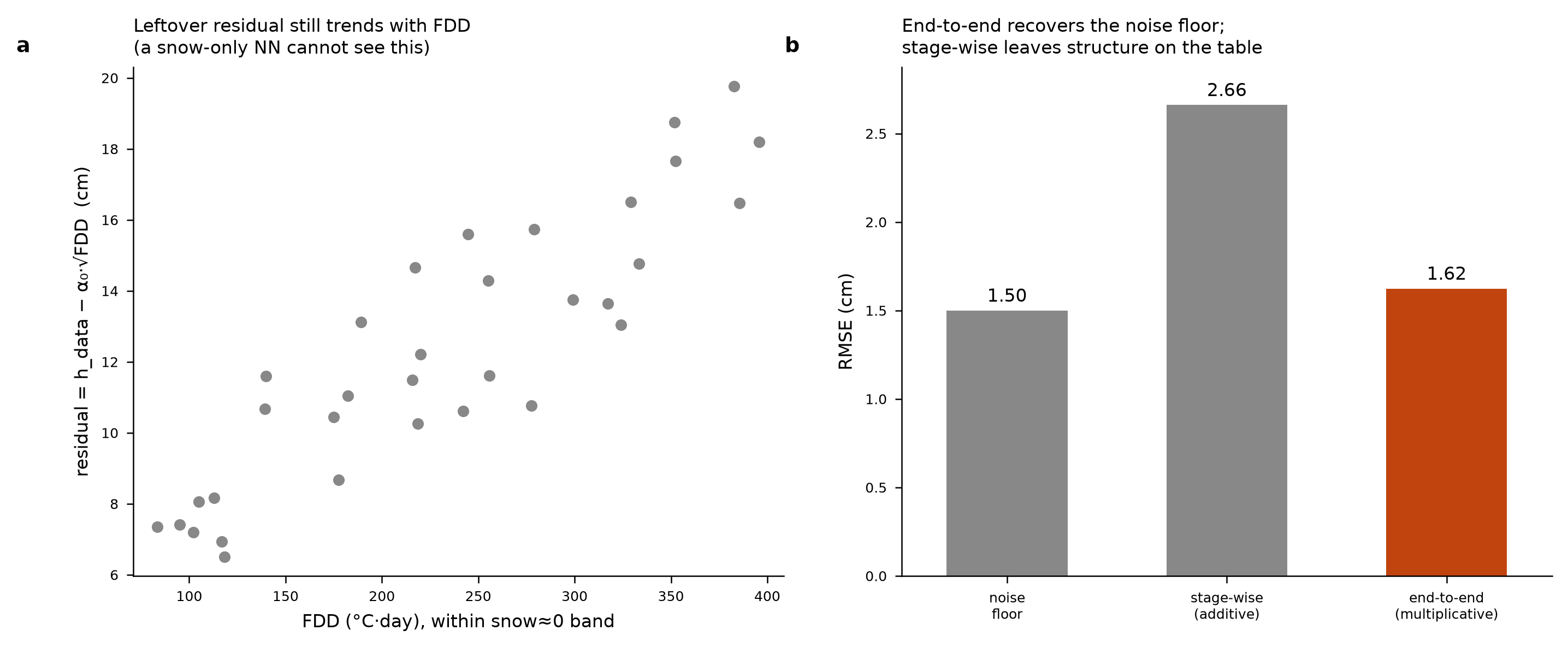
Stage-wise split: leftover residual still trends strongly with FDD

Figure 5. Why a stage-wise split loses accuracy. Left: within a narrow low-snow band, the residual left by a fixed \(\alpha_0\) = 2.6 still trends strongly with \(FDD\) (r ≈ 0.89) — structure a snow-only stage-2 network cannot see. Right: RMSE comparison — end-to-end (1.62 cm) nearly reaches the noise floor (1.50 cm), while the additive stage-wise split stalls at 2.66 cm because the true interaction is multiplicative.

Within that narrow snow band the residual correlates strongly with \(FDD\) (r ≈ 0.89) — but the stage-2 network is fed only snow, so it structurally cannot see or correct that \(FDD\)-dependent trend. It is forced to collapse to a per-snow average, discarding the spread. That discarded spread is the gap between 1.62 and 2.66 cm.

The general principle: a stage-wise split is safe only when the unknown closure enters additively and independently of the physics — \(h = physics(FDD) + f(\text{snow})\). The moment the closure interacts with the physics (multiplication, thresholds), a fixed split point bakes in an error that no amount of stage-2 retraining can undo, because stage 2 never sees the variable it would need. Real ice closures (frazil formation, snow insulation, under-ice heat flux) interact multiplicatively with the physics-component state, so this is the rule rather than the exception — which is the substantive reason to want genuine end-to-end differentiability rather than a sequential physics-then-patch design.

3b. Neural-network basics: what the layers actually are

The architecture Linear, Tanh, Linear, Softplus is built from a small standard menu:

Linear(m, n) — the only piece with learnable weights: output = W·input + b. You choose how many and how wide (the 16s in Example 3 are a capacity choice, not a fixed rule).
Activation functions (Tanh, Softplus, ReLU, Sigmoid, …) — fixed, hand-picked nonlinear functions with no learnable parameters. The menu is genuinely short; picking among them is largely convention.

Why the activations are load-bearing: stacking Linear layers with nothing between them collapses to a single Linear layer — I checked, and three stacked linear layers equal one collapsed matrix product to floating-point noise (max difference 1.5e-08). Matrix products compose into one matrix. The Tanh nonlinearities are what stop the collapse and give the network the ability to represent curved relationships like 3.5 − 1.8·snow. The final Softplus serves a different purpose: keeping the output physically valid (\(\alpha\) > 0).

3c. Three ways to train the same network — and what is actually required

There are two different things loosely called “gradient”: (1) the per-weight gradient \(\partial \text{Loss}/\partial weight\) that training needs, and (2) the inter-layer gradients that the chain rule produces as intermediate scratch values. Only #1 is fundamentally required — and even that only if you choose a gradient-based method. To convince myself, I trained the identical closure three ways:

method	uses inter-layer gradients?	uses per-weight gradient?	final loss
1. Backprop (chain rule) + Adam	yes (as intermediates)	yes	2.40
2. Finite-difference + Adam	no (treats NN as black box)	yes (approximated)	2.38
3. Derivative-free search	no	no gradients at all	2.22

All three reach the noise floor (2.25).

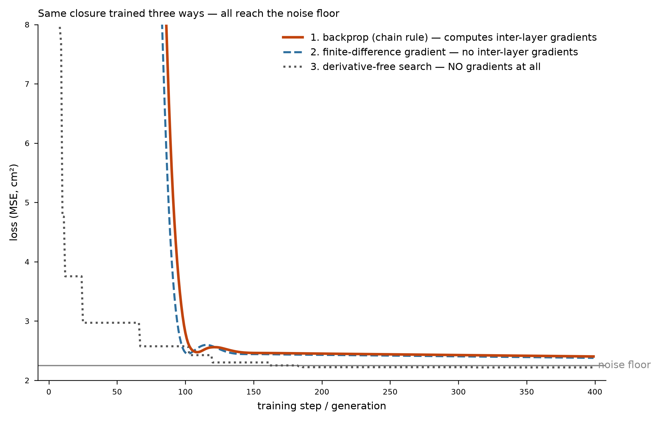
Three training methods all converging to the noise floor

Figure 6. The same 321-parameter closure trained three ways — backprop + Adam, finite-difference + Adam, and derivative-free search — all converge to the same noise floor (~2.25). The methods are equivalent in outcome; they differ only in cost: backprop returns every gradient in one backward pass, finite differences needs 642 passes per step, and derivative-free search needs a whole population per step.

Method 2 gets each weight’s gradient by poking it (nudge up, nudge down, re-run) — never looking inside the network. So the inter-layer gradients are not required; they are just how backprop happens to compute the per-weight gradient cheaply.
Method 3 uses no gradients whatsoever — sample small random weight changes, keep whatever lowers the loss. This is essentially the SCE/DDS family. It still trains the network.

So what is required? Only a way to keep adjusting weights so the loss goes down. Nothing more. The three methods differ entirely in cost scaling:

Backprop returns all per-weight gradients in one backward pass, regardless of network size, by reusing the inter-layer intermediates. For Example 3’s 321-parameter network: 1 forward + 1 backward.
Finite differences costs 2 forward passes per weight — 642 passes per step for that same network.
Derivative-free search needs a whole population of evaluations per step, growing with parameter count.

This is the same cost-scaling story as SCE-vs-gradient-descent from Example 2, one level deeper: for a handful of physical constants, any method works. For a large regionalized closure with hundreds-to-millions of weights, backprop is the only one that stays affordable. That is the entire practical reason “differentiable” ML matters — not elegance, but the ability to get every gradient essentially for free.

3d. Is the neural network really a “black box”? (No.)

A common mental model is that .backward() stops at the network’s boundary and treats it as one opaque unit. It does the opposite — it traverses every operation inside the network. To see this for myself, I printed PyTorch’s own recorded computation graph (loss.grad_fn) for the Example-3 forward pass:

MeanBackward0        (loss = mean(sq))
PowBackward0         (sq = diff²)
SubBackward0         (diff = h_pred − h_obs)
MulBackward0         (h_pred = alpha · √FDD)   <- the physics↔NN seam
SoftplusBackward0    <- inside the NN: Softplus layer
AddmmBackward0       <- inside the NN: 2nd Linear layer
TanhBackward0        <- inside the NN: Tanh layer
AddmmBackward0       <- inside the NN: 1st Linear layer
AccumulateGrad ×4    <- the leaf weight/bias tensors (what Adam updates)

Every layer of the “black box” appears as its own node. The seam between physics and network — the link \(\partial h_{pred}/\partial \alpha = \sqrt{FDD}\) — is not a place where tracing stops or restarts; it is just one more link in an unbroken chain that autograd walks identically on both sides.

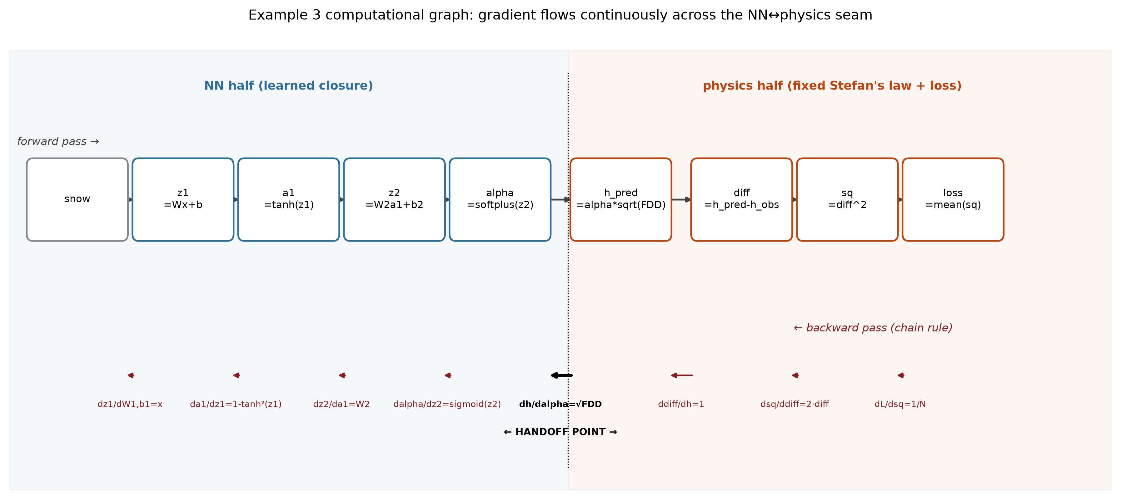
The physics-NN seam as one unbroken chain, forward and backward

Figure 7. The physics↔NN seam as one unbroken chain. Forward pass runs left-to-right (snow → NN → \(\alpha\) → ×\(\sqrt{FDD}\) → \(h_{pred}\) → loss); the backward pass runs right-to-left with the local derivative labeled on every link. The seam \(\partial h_{pred}/\partial \alpha = \sqrt{FDD}\) is just one more link — autograd walks the NN side identically to the physics side.

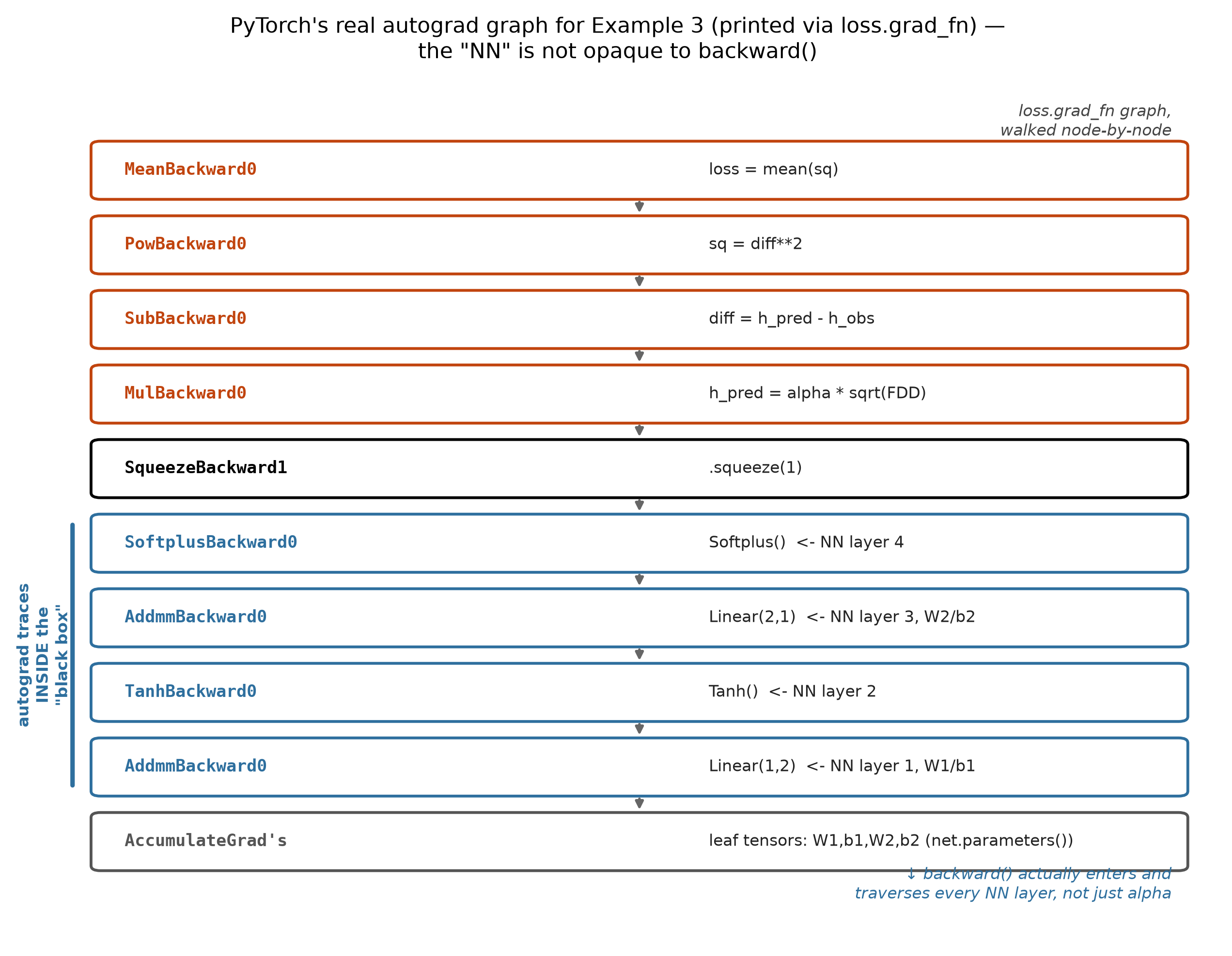
PyTorch's real autograd graph, walked node-by-node

Figure 8. PyTorch’s actual recorded computation graph for the Example-3 loss, walked node-by-node from MeanBackward0 down to the four AccumulateGrad leaf tensors. Every internal NN layer (Softplus, the two Linear/Addmm layers, Tanh) appears as its own node — proof that .backward() traverses inside the network rather than stopping at its boundary.

I confirmed the numbers too: on a tiny 3-point, 2-hidden-unit version, every gradient computed by hand (chain rule) matched autograd to 5+ significant figures — including the gradient crossing the seam (\(\partial \text{Loss}/\partial \alpha\)) and the deepest weight gradients (\(\partial \text{Loss}/\partial W1\), \(\partial \text{Loss}/\partial b2\) = -191.22). The “black box” framing is true only in the sense that you don’t have to write the calculus yourself — computationally, autograd has full-depth visibility into every weight.

Why this matters: end-to-end training is possible only because autograd treats physics operations and NN-layer operations as the same kind of thing — nodes in one graph, each contributing a local derivative. If the network really were opaque to gradients, you would be forced back into the stage-wise split of Section 3a, with the information loss that entails.

The broader Earth-system-modeling landscape

None of this is my invention — the Example-3 pattern (trusted differentiable physics + learnable closures, trained end-to-end) is the organizing idea behind a fast-growing body of Earth-system work. Here are the landmarks I keep coming back to, mapped onto the toy version above:

NeuralGCM (Kochkov et al., Nature, 2024) — a differentiable atmospheric general-circulation model. A conventional dynamical core (solving the fluid-dynamics equations for large-scale flow) is coupled to neural networks that learn the unresolved sub-grid physics — convection, clouds, radiation — the very closures that are hand-tuned in traditional GCMs. Trained end-to-end against reanalysis, it matches or beats conventional models on medium-range and climate timescales at far lower cost. This is Example 3 at planetary scale: \(\sqrt{FDD}\) → the fluid dynamical core; \(\alpha(\text{snow})\) → the learned convection/cloud closures.
Differentiable hydrology (δHBV, HBV-type + NN; Feng, Shen and colleagues) — the closest analog to my MOSART goal. A differentiable conceptual rainfall–runoff model keeps the mass-balance structure (buckets, routing) as the physics component and learns its parameters as functions of static catchment attributes via an embedded network — trained across many basins simultaneously (regional / “big-data” calibration). This is precisely the staged, regionalized calibration strategy that motivates differentiability over per-basin SCE: you are learning a parameter field over attribute space, which has far too many effective degrees of freedom for population search.
Process-guided / hybrid lake models — deep-learning lake-temperature and ice models that embed energy conservation or known thermodynamic constraints as physics terms alongside learned components, improving generalization to unmonitored lakes. Directly adjacent to the lake-ice framing of this document.
My MOSART river/lake-ice application — the concrete target. Stefan-type ice growth (and the fuller River1D-style heat/frazil/border-ice process set) is the differentiable physics component; the empirical closures (Stefan coefficient as a function of snow and other attributes, frazil and border-ice rules, composite roughness) become learnable functions, calibrated regionally across many basins against observed ice thickness, breakup timing, and discharge. Section 3a is the warning label: because those closures interact multiplicatively and through thresholds with the physics-component state (discharge, water temperature, ice concentration), a sequential physics-then-ML-patch design will leave recoverable error on the table — the reason to build it end-to-end from the start. Hard on/off rules (Froude-number gates, under-cover cutoffs) must be smoothed (sigmoid/softplus) before gradients can flow through them — the one genuine engineering caveat carried over from the River1D reading.

The common thread: in every case the modeler keeps the equations they trust, isolates the parts they don’t, makes the whole thing differentiable, and lets gradients trained on observable outputs teach the uncertain closures — with the size of the learnable part being exactly what makes differentiability non-optional.

Appendix — companion Jupyter notebook

A fully commented, runnable notebook reproducing all three examples plus the two “extra” experiments (stage-wise vs. end-to-end; three ways to train) is saved alongside this post:

diffml_lake_ice_examples.ipynb

Every code cell has been executed and verified to reproduce the exact numbers quoted above. Fixed seeds: torch.manual_seed(0) for Example 2, torch.manual_seed(1) for Example 3 and the extras, torch.manual_seed(7) for the tiny hand-trace network. Environment: Python 3.11, PyTorch 2.x, NumPy, Matplotlib.

Reproduction note: all figures were generated from the same fixed-seed code as the notebook. If you re-run and see numbers differing in the last decimal, check your PyTorch version — the random-number stream is version-stable but not guaranteed identical across major releases.